Использование битовой маски для выбора хеша
Теперь, когда у него есть хеш, что Postgres делает с ним? Вы можете увидеть подсказку выше в комментариях C:
Наилучшие размеры хеш-таблиц — степени 2. Нет необходимости делать мод простыми (мод очень медленный!). Если вам нужно менее 32 бит, используйте битовую маску.
Хеш-таблица состоит из массива «сегментов», которые представляют собой серию указателей на связанные списки. Первоначально Postgres создает пустой массив указателей сегментов непосредственно перед началом сканирования публикаций:
Как вы можете догадаться, Postgres сохраняет каждую публикацию в одном из сегментов в хеш-таблице на основе вычисленного хеш-значения. Позже, когда он просмотрит авторов, он сможет снова быстро найти публикации, пересчитав те же хеш-значения. Вместо того, чтобы снова сканировать все публикации, Postgres может просто искать автора каждой публикации, используя хеш. Хеш — это запись о том, где каждая публикация сохраняется в хеш-таблице.
Однако, если у двух публикаций окажется один и тот же автор, как у нас в нашем примере, то Postgres должен будет сохранить их обе в одной корзине. Вот почему каждый сегмент представляет собой связанный список; каждое ведро должно сохранять более одной публикации.
Поскольку в нашем примере три публикации, использует ли Postgres хеш-таблицу с тремя сегментами? Или с двумя ведрами, из-за повторного значения автора? На самом деле он использует 1024 ведра! Почему 1024? По двум причинам: во-первых, Postgres был разработан для запроса больших объемов данных. Его алгоритм хеш-соединения был оптимизирован для обработки очень больших наборов данных, содержащих миллионы записей или даже больше. Таблица, содержащая три записи, действительно крошечная! Postgres не заботится о небольших хеш-таблицах и использует минимальный размер 1024.
И почему степень двойки? Это облегчает определение того, какой сегмент использовать для данного хэша. Вместо того, чтобы пытаться возвращать хеш-значения, соответствующие количеству сегментов, проще и быстрее всегда возвращать очень большие значения. Вместо этого Postgres распределяет большие хэш-значения равномерно по количеству сегментов, которые у него есть. Выбирая степень двойки для размера массива сегментов, Postgres может использовать быструю побитовую операцию, чтобы решить, в какой сегмент сохранять каждую публикацию, например:
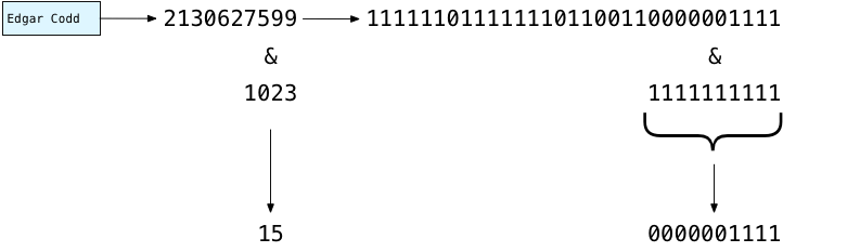
Выше вы можете увидеть, как Postgres решает, куда поместить «Эдгар Кодд» в хеш-таблицу: он вычитает одно из числа сегментов: 1024-1 = 1023. Записывается в двоичном виде это 1111111111. Затем с помощью бинарных вычислительных схем вашего микропроцессора, Postgres быстро маскирует левые биты и сохраняет только 10 наименее значимых или самых правых битов. В результате получается двоичный код 0000001111 или число 15. Используя этот быстрый расчет, Постгрес решает сохранить Эдгара в корзине № 15:
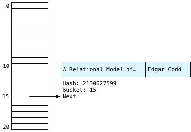
Postgres также сохраняет строку заголовка, потому что она понадобится позже для получения окончательного набора результатов. Наряду с двумя строками Postgres сохраняет значение хеш-функции и указатель «следующий», который сформирует связанный список.
Создание остальной части хеш-таблицы
Postgres теперь продолжает просматривать публикации, придя ко второй публикации.
У нас снова Эдгар! Очевидно, он был центральной фигурой в теории баз данных. При повторном вычислении хеша для одной и той же строки всегда будет возвращаться одно и то же значение: 2130627599, в результате получится контейнер № 15 во второй раз. Мы знаем, что записи Эдгара Кодда всегда будут появляться в 15-м ведре.
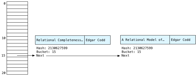
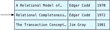
Также обратите внимание, что Postgres сохраняет каждую новую публикацию во главе связанного списка — это означает, что у нас вторая вторая публикация Эдгара первая слева, а первая публикация Эдгара вторая справа. Как мы увидим далее, это дает обратный порядок записей Эдгара, которые мы видели выше в концептуальном алгоритме.
Наконец, Postgres продолжает сканирование и сохраняет третью публикацию в хеш-таблице; на этот раз Postgres вычисляет хеш для «Джим Грей:»
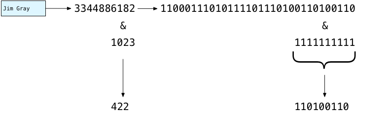
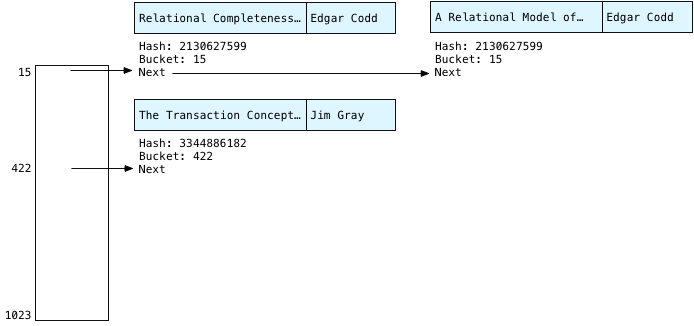
You can see this time the 10 rightmost bits of 3344886182 evaluate to 422. So, Postgres saves Jim in bucket #422. Drawing the bucket array more to scale it might look something like this:
Scanning Buckets
After saving all the publications in the hash table, Postgres can now scan over the authors table:
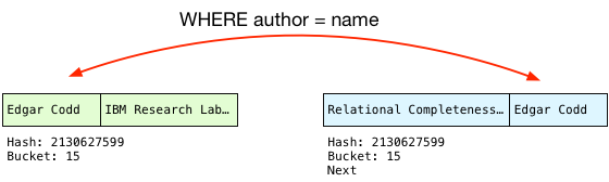
Now, finding the matching publication is simple. Instead of scanning over all the publications, Postgres simply calls the hash function again on the name string from the authors table, and repeats the bitmask operation. Because the first author record is Edgar, Postgres knows the matching publications will be in bucket #15.
In our tiny example, the only records in bucket 15 will be for Edgar Codd. But, remember in a large SQL query there might be millions of publications. It’s possible that publications with different authors might appear in this bucket. This would happen because either:
- The hash function returned the same hash number for two different author strings. This is possible but unlikely. In Computer Science this would be known as a hash collision.
- The 10 least significant bits of the hash were the same. For millions of publications this would happen frequently. However, as the number of records in the join increases Postgres uses more and more bits in the bitmask. 1024 (10 bits) was the minimum number it uses for our tiny query. Still, hash table buckets in practice will contain multiple key values.
Therefore, Postgres has to check each author in the matching bucket to be sure that it’s a match. This process is known as scanning the bucket. To do this, Postgres first checks the hash values:
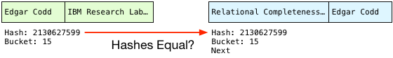
This is a simple numerical comparison and so is quite fast. And if the hashes are the same, Postgres checks the actual strings just in case the hash function did return the same hash for different strings:
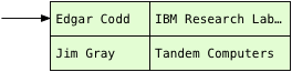
Because the author names match, Postgres can finally perform the join! To do this, it projects the columns that our query selects into a single joined record, in the desired order:
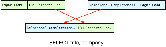
This becomes the first record in our result set.
Returning Multiple Records: The Hash Join State Machine
One of the most beautiful and important aspects of the Postgres implementation is the way it orchestrates building up and searching the hash table in the midst of a larger enclosing SQL expression. To see this for yourself, take a look at the hash join implementation, in nodeHashJoin.c.
(«ExecHashJoin» method — view on postgresql.org)
Postgres calls ExecHashJoin once for each record in the join result set. For our example with 3 result records, Postgres calls ExecHashJoin three times. ExecHashJoin keeps track of how many times it has been called, and what it needs to do next, using a state machine.
The best way to understand how this state machine works, and how it fits into the larger structure of Postgres’s architecture, is to imagine that we asked for one record at a time. For example, imagine that we select just a single record from the join:
select title, company from publications, authors where author = name limit 1
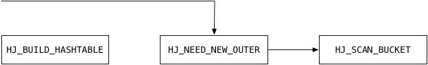
By appending limit 1 we tell Postgres to stop after 1 record. For this query, to return just one record, ExecHashJoin will use the following states in its state machine:

Here’s what ExecHashJoin does to obtain the first joined record:
- HJ_BUILD_HASHTABLE: This code builds the hash table by scanning over all the publications records, as we saw above. Postgres calls publications the “inner relation.”
- HJ_NEED_NEW_OUTER: This code starts scanning the “outer relation” or the authors table in this example, and returns a single record.
- HJ_SCAN_BUCKET: This code takes one outer relation record (an author) and looks for the matching inner relation records in the hash table (publications).
Now, imagine that I ask Postgres for two records, by using limit 2:
select title, company from publications, authors where author = name limit 2
The second time Postgres calls ExecHashJoin, it only executes HJ_NEED_NEW_OUTER and HJ_SCAN_BUCKET – it already created the hash table the first time it was called:
Postgres pays the large price of scanning the entire inner relation and building the hash table as soon as you ask for one record. Returning the second and all subsequent records is much faster because Postgres already has the hash table.
If you read the C code, you’ll see some interesting optimizations. For example, Postgres actually scans the outer relation first to get a single record, just in case it might be empty. (This is what the C comment above refers to.) There’s no need to build a hash table if we’re not going to look up any values! Also, the HJ_FILL_INNER and HJ_FILL_OUTER states handle executing right or left outer joins respectively. ExecHashJoin implements these as well.
By using a state machine like this Postgres can execute this join inside the context of a large, complex SQL statement. It could be that we are joining together result sets from complex inner SQL clauses, or that the result set from this join becomes part of a larger expression. The state inside of ExecHashJoin allows Postgres to keep track of what it was doing–and of what it needs to do next–in the appropriate place on the execution stack.
What’s Next?
The last state value handled by ExecHashJoin, HJ_NEED_NEW_BATCH, handles the case where the hash table doesn’t fit into the server’s memory. In this case, Postgres will create a series of hash tables and save some of them out to disk in “batch files.” This algorithm is what the term Hybrid Hashjoin refers to.
When I have time, I’d love to write about how Postgres handles a large join instead of a tiny one: How do batch files work? What configuration settings have an effect on batch files and join performance? And there’s also an interesting optimization Postgres uses for frequently occurring join key values.
Postgres does some amazing things internally to speed up your queries; it’s time to shed some light on the great work the Postgres open source community has done over the years!
(Make sure to read part 1 if you haven’t already.)