Эта статья является краткой версией моего поста из пяти частей.
После недолгой работы с базами данных RDF, SPARQL и Virtuoso мне стало интересно, как на самом деле работают графовые базы данных. У меня есть опыт использования баз данных и представление о том, как они работают внутри, но редко требуется тщательный анализ их внутренней работы. В этом посте я попытаюсь лучше понять как реляционные, так и графовые базы данных. Мой главный вопрос: как именно графические базы данных работают лучше, чем реляционные базы данных для связанных данных? То, как они хранят данные, делает их такими хорошими? Или есть какой-то магический алгоритм, который делает графические базы данных очень удобными.
Два типа графовых баз данных
Во время чтения потребовалось некоторое время, прежде чем я понял, что существует как минимум два вида графовых баз данных: графовые базы данных, основанные на реляционных базах данных (например, тройные хранилища ) и собственные графовые базы данных. Мой анализ основан на сравнении баз данных собственных графов (прежде всего Neo4j) с реляционными базами данных. Смотрите мой пост, чтобы получить краткое сравнение двух.
Почему и когда использовать базы данных графиков
Первое, что я сделал, было в Google в целом о графовых базах данных и моем вопросе. Графовые базы данных хорошо подходят для сильно связанных данных, которые хорошо вписываются в графическую структуру. Я нашел причины, по которым графические базы данных лучше подходят для связанных данных, чем реляционные базы данных:
- Better performance – highly connected data can cause a lot of joins, which generally are expensive. After over 7 self/recursive joins, the RDMS starts to get really slow compared to Neo4j/native graph databases.
- Flexibility – graph data is not forced into a structure like a relational table, and attributes can be added and removed easily. This is especially useful for semi-structured data where a representation in relational database would result in lots of NULL column values.
- Easier data modelling – since you are not bound by a predefined structure, you can also model your data easily.
- SQL query pain – query syntax becomes complex and large as the joins increase.
Points 2, 3 and 4 are easy to agree with, at least with in my experience. The thing that caught my eye was the better performance feature of graph databases. I wanted understand what kind issues the joins are causing which make them slower compared to traditional relational databases. More specifically, why does adding more joins make RDMS slower. Since joins play a vital role in comparing graph databases with relational databases performance, I will look into two common join algorithms to compare them with the graph database approach.
Two Join Approaches: Nested Loop and Hash Join
A DBMS can join in many different ways and two of the most common ones are nested loop join and hash join. All joins are performed two tables at a time, even if more tables are described in the query. This means that in cases with more than two join-tables, intermediary steps are required because the result of first join must be used joined with the third. This again impacts the performance.
Nested Loop Join
Nested loop join is the simplest of the joins where the join is performed by, as the name suggests, nested loops. For each row in the inner table, all rows of the outer table are read. If the join is extended for more tables, the time complexity increases drastically. Nested loop join is only good for small tables or where the final result of the query is small. Indexes are used if they exist on the join column, and this will benefit performance. The following example for a nested loop join between two tables employees and departments, is taken from the Oracle documentation:
FOR erow IN (select * from employees where X=Y) LOOP
  FOR drow IN (select * from departments where erow is matched) LOOP
    output values from erow and drow
  END LOOP
END LOOP
If an index is useful in the outer loop due to the where condition or in the inner loop due to index on join column, it will be used. Regardless, the inner loop is run for each row from the outer loop. So, as the joins increase, the nested loops increase and when indexes are used, we avoid the worst case which is time complexity proportional to table sizes (|employees|*|departments|). But, even if indexes are used the complexity still increases and can increase non-linearly, which means it get slower and slower as more joins are added.
Hash Join
Hash join prepares a temporary hash table of the smaller table before joining. It then traverses the larger table one time, while doing a lookup in the temporary hash table to find matches. For this to work best, the smaller data set should fit in main memory. Hash joins do not benefit from indexes on join columns because of the temporary hash table. The Oracle example for hash join is
FOR small_table_row IN (SELECT * FROM small_table)
LOOP
  slot_number := HASH(small_table_row.join_key);
  INSERT_HASH_TABLE(slot_number,small_table_row);
END LOOP

FOR large_table_row IN (SELECT * FROM large_table)
LOOP
   slot_number := HASH(large_table_row.join_key);
   small_table_row = LOOKUP_HASH_TABLE(slot_number,large_table_row.join_key);
   IF small_table_row FOUND
   THEN
      output small_table_row + large_table_row;
   END IF;
END LOOP;
Time complexity for hash joining two tables employees (larger) and departments (smaller), is the sum of :
- Time for creating temporary hash table for departments which requires reading of all the rows in departments + creation of the hash table (first for loop)
- Time for calling the hash function to fetch the matching join row, for each row in employees (second for loop).
If more joins are added then this procedure must be repeated because of intermediary joins – i.e. create new hash table based on the result of current join to join with the third table. Based on this, it is possible to conclude that hash join gives linear complexity increase as the joins increase. However the actual time may be non-linear because of intermediary join steps, hash table constructions and hash lookups which are very dependent on the data. It is therefore not easy to give a general conclusion on how hash joins effect performance, but we do get an indication.
Comparing Joins With Graph Database Approach
So, why are joins not a problem for Neo4j? The neat thing about Neo4j is that it does not use indexes at all. Instead, graph nodes are linked to its neighbors directly in the storage. This property of reference is called index-free adjacency. So, when Neo4j performs a graph query for retrieving a sub-graph, it simply has to follow the links in the storage – no index lookups are needed. The cost of each node-to-node traversal is O(1) – so if we are doing a friend-of-a-friend look-up to find, for example, all indirect friends of Alice, the total cost would be proportional to total number of friends in the final result – O(m) where m is the total number of Alice’s indirect friends. Even if the data (number of nodes) increases, if the total number of friends are still the same, the cost will still by O(m). This is because Neo4j first “jumps” to the Alice node using some kind of search or index, and then it simply visits the relating nodes by following the links, until the query is satisfied .
To compare the graph database approach with RDMS we will go through a simple example. Assume that we have tables Employees (E), Departments (D) and Payments (P).
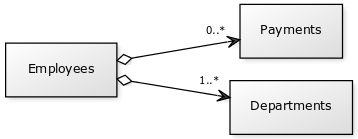
By joining E with D and then E with P, we can calculate for example sum payment for a given department. Given departments d1 and d2, we want to find all the payments to its employees. By using nested loop join, this approach has a time complexity cost proportional to 2 * |E| * |P| (2 for two departments, as we assume that an hash index is used to retrieve the d1 and d2). Using hash join, this gives a a time complexity cost proportional to 2 +|E|+2*|E|+|P|, where 2+|E| is the first join, and 2*|E|+|P| is the second. Again, the first 2 is for retrieving d1 and d2, while |E| is for looping the larger table. 2*|E| is the number of maximum rows that can be constructed by joining d1 and d2 with E. The |P| is the final looping of each row to find corresponding employee in the first joined set, and to create joined rows.
A subset graph of our example is as follows:
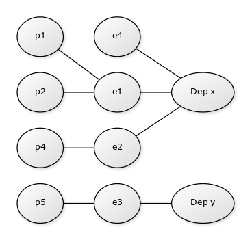
where e’s are employees and p’s are payments.
To find the payments with Neo4j, first a search is conducted to find the departments d1 and d2. Using hash indexing this gives O(1). Then the graph is “walked” to find all the relevant payments, by first visiting all employees in the departments, and through them, all relevant payments. If we assume that the number of payment results are k, then this approach takes O(k). We now have the following time complexities for our query (simplifying the according to Big-O notation):
- nested loop join:
O(|E| * |P|) - hash join:
O(|E|+|P|) - Neo4j:
O(k)
Two conclusions can be drawn from these:
- As the amount of rows increases in
EandP, the nested loop join and hash join cost will increase, while Neo4j cost is the same. If index are used to pinpoint the correct datasets, the database still needs to search the index. This takesO(log(n))for B+ trees, a number that also increases as the data is added, although slowly (in practice, the growth is often not a problem). Using hash index, this search may be reduced toO(1), but hash indexes are often difficult to scale, don’t support range queries and rebuilding indexes takes a lot of time , so B+trees are more common. Neo4j cost is not dependent of the amount of data, thus it stays the same. So, if millions of new rows were added to all the tables, both RDMS join approaches will suffer resulting in slower performance, while the graph database performance will be almost the same (except the first search after departmentsd1andd2). - If we add more intermediary nodes in the graph, corresponding to new tables in the joins, both approaches suffer, but RDMS cost can increase non-linearly. As an example we can add a new table called PaymentItem (
PI) which describe some detail for a payment, and change our query to find payment items related to departments. The graph database would now have to “walk” a longer distance to perform the query, but because the graph database walk started from the correct departments, it will only consider the relevant payment items, instead of all. For RDMS, another table will be added to the joins and the cost change toO(|E| * |P| * |PI|)for nested loop join, andO(|E|*|P|+|PI|)for hash join (proportional to2 +|E|+2*|E|+|P|+2*|E|*|P|+|PI|). These cost are non-linear and much larger than for graph! Thus, adding new table relations in RDMS can result in non-linear performance increase in worst case.
Note that these conclusion describe the worst case and in practice, by tuning and optimizing, the cost for using RDMS can be heavily reduced.
Sources
- Robinson, I., Webber, J. & Eifrem, E. book: Graph databases (2013) O’Reilly Media
- Use the Index, Luke: http://use-the-index-luke.com/sql/join
- Oracle documentation on database indexes.
- Ramakrishnan, Raghu, and Johannes Gehrke book: Database management systems (2003) slides from chapter 12
Related Work
Analysis in this post is of course a very simple one, and was mostly conducted to understand the underlying details. In my research, I did a survey find others say about Neo4j performance which is listed below. In summary, I find that Neo4j generally do outperform RDBMS, but there are cases where this does not happen. The lesson learned is that graph database field is still very young as lots of development and research is happening there. This implies that when someone considers a graph database, performance tests should be conducted to verify that the database actually performs well for their data.
- Vicknair, Chad, et al. “A comparison of a graph database and a relational database: a data provenance perspective.” Proceedings of the 48th annual Southeast regional conference. ACM, 2010.
- This comparison between Neo4j and MySQL is from 2010 and shows that Neo4j performs well on queries involving graph traversals and text search. However, MySQL has performs similar to Neo4j on queries for orphan nodes, and outperforms Neo4j for queries involving integer payload (e.g. Count the number of nodes whose payload data is less than some value).
- https://baach.de/Members/jhb/neo4j-performance-compared-to-mysql/view
- This is also a comparison between Neo4j and MySQL where the author is examining the performance claims from the Graph databases book by redoing the queries from the book. Here, the author manages to get better results with MySQL than Neo4j on friend-of-a-friend graph, and he is unsure of why.
- De Abreu, Domingo, et al. “Choosing between graph databases and rdf engines for consuming and mining linked data.” Proceedings of the Fourth International Conference on Consuming Linked Data-Volume 1034. CEUR-WS. org, 2013.
- This is a performance comparison of graph databases DEX, Neo4j, HypergraphDB and RDF-3x where they conclude with that none of the graph databases are superior the other in all graph based tasks. Neo4j has
a better performance in BFS and DFS traversals, as well as in mining tasks against sparse large graphs with high number of labels.
- Martínez-Bazan, Norbert, et al. “Efficient graph management based on bitmap indices.” Proceedings of the 16th International Database Engineering & Applications Sysmposium. ACM, 2012.
- Here, the authors describe the internals of the graph database DEX and the clever usage of bitmap indexing in their graph model. In their experiments, DEX outperforms Neo4j on the queries they tested. More interesting is that, even MySQL outperforms Neo4j in their tests!