Как вы могли заметить — по крайней мере, если вы читали объяснение производительности SQL — я не думаю, что кластерные индексы столь же полезны, как считает большинство людей. Это в основном потому, что слишком сложно выбрать хороший ключ кластеризации. На самом деле, выбрать хороший, «правильный» ключ кластеризации практически невозможно, если в таблице более одного или двух индексов. В результате большинство людей просто придерживаются значения по умолчанию, которое является первичным ключом. К сожалению, это почти всегда худший из возможных вариантов.
В этой статье я объясняю зверя с именем кластеризованный индекс и все его недостатки. Хотя эта статья использует SQL Server в качестве демонстрационной базы данных, эта статья в равной степени относится и к MySQL / MariaDB с InnoDB и к базе данных Oracle при использовании таблиц, организованных по индексу.
Резюме: что такое кластерный индекс
Идея кластерных индексов состоит в том, чтобы хранить полную таблицу в структуре B-дерева. Если таблица имеет кластерный индекс, это в основном означает , что индекс являетсяТаблица. Кластерный индекс имеет строгий порядок строк, как и любой другой индекс B-дерева: он сортирует строки в соответствии с определением индекса. В случае кластеризованных индексов мы называем столбцы, которые определяют порядок индекса, ключом кластеризации. Альтернативный способ хранения таблицы — это куча без определенного порядка строк. Кластерные индексы имеют то преимущество, что они поддерживают очень быстрое сканирование диапазона. То есть они могут быстро извлекать строки с одинаковым (или похожим) значением ключа кластеризации, поскольку эти строки физически хранятся рядом друг с другом (кластеризовано), часто на одной странице данных. Когда дело доходит до кластерных индексов, очень важно понимать, что нет отдельного места, где хранится таблица. Кластерный индекс являетсяхранилище первичной таблицы — таким образом, вы можете иметь только одну таблицу на таблицу. Это определение кластерных индексов — это отличие от таблиц кучи.
Однако существует другой контраст с кластеризованными индексами: некластеризованные индексы. Именно из-за именования для многих это более естественный аналог кластеризованных индексов. С этой точки зрения основное отличие заключается в том, что запрос кластеризованного индекса всегда выполняется как сканирование только по индексу. Некластеризованный индекс, с другой стороны, имеет только подмножество столбцов таблицы, поэтому он вызывает дополнительные операции ввода-вывода для получения недостающих столбцов из хранилища первичных таблиц, если это необходимо. Для этой цели каждая строка в некластеризованном индексе имеет ссылку на одну и ту же строку в хранилище первичной таблицы. Другими словами, использование некластеризованного индекса обычно подразумевает устранение дополнительного уровня косвенности. Вообще я сказал. На самом деле, это довольно легко избежать, если включить все необходимые столбцы в некластеризованный индекс.В этом случае база данных может найти все необходимые данные в индексе и просто не разрешает дополнительный уровень косвенности. Даже некластеризованные индексы можно использовать для сканирования только по индексам, что делает их такими же быстрыми, как кластерные индексы. Разве это не главное?
Запись
Важным понятием является сканирование только по индексу, а не кластерный индекс.
Позже в этой статье мы увидим, что между этими аспектами кластеризованных индексов есть двойственность: быть хранилищем таблиц (в отличие от таблиц кучи) или индексом, который имеет все столбцы таблицы. К сожалению, эта «двойственность табличного индекса» может быть столь же запутанной, как и дуальность волны и частицы света . Следовательно, я буду четко указывать, какой аспект появляется в то время, когда это необходимо.
Расходы на дополнительный уровень косвенности
Когда дело доходит до производительности, дополнительный уровень косвенного обращения не совсем желателен, потому что разыменование требует времени. Важным моментом здесь является то, что стоимость разыменования сильно зависит от способа физического хранения таблицы — либо в виде таблицы кучи, либо в виде кластерного индекса.
Следующие цифры объясняют его феномен. Они визуализируют процесс выполнения запроса для извлечения всех SALESстрок с 2012-05-23. На первом рисунке используется некластеризованный индекс SALE_DATEвместе с таблицей кучи (= таблица без кластеризованного индекса):
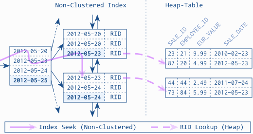
Обратите внимание, что существует одна Index Seek (Non-Clustered)операция над некластеризованным индексом, которая приводит к двум RID Lookupsв таблице кучи (по одной для каждой подходящей строки). Эта операция отражает разыменование дополнительной косвенной ссылки для загрузки оставшихся столбцов из хранилища первичных таблиц. Для таблиц кучи некластеризованный индекс использует физический адрес (так называемый RID) для ссылки на ту же строку в таблице кучи. В худшем случае дополнительный уровень косвенности приводит к одному дополнительному доступу на чтение на строку (игнорируя пересылку).
Теперь давайте посмотрим на тот же сценарий с кластерным индексом. Точнее говоря, при использовании некластеризованного индекса в присутствии кластеризованного индекса, SALE_IDто есть первичного ключа в качестве ключа кластеризации.
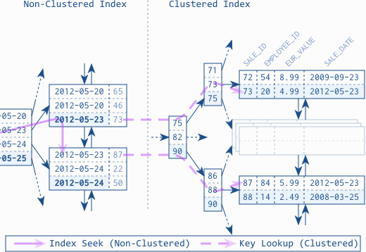
Обратите внимание, что определение индекса слева не изменилось: это все еще некластеризованный индекс SALE_DATE. Тем не менее, чистое присутствие кластеризованного индекса влияет на то, как некластеризованный индекс относится к хранилищу первичной таблицы, а именно к кластерному индексу! В отличие от таблиц кучи, кластеризованные индексы являются «живыми существами», которые перемещают строки по мере необходимости, чтобы поддерживать свои свойства (то есть: порядок строк и баланс дерева). Следовательно, некластеризованный индекс больше не может использовать физический адрес в качестве ссылки, поскольку он может измениться в любое время . Вместо этого он использует ключ кластеризации в SALE_IDкачестве ссылки. Загрузка отсутствующих столбцов из хранилища первичной таблицы (= кластеризованный индекс) теперь включает полный обход B-дерева для каждой строки. Это несколько дополнительные операции ввода-вывода на строку в отличие от одного дополнительного ввода-вывода в случае таблиц кучи.
Я также называю этот эффект «штрафом за кластерный индекс». Это наказание влияет на все некластеризованные индексы в таблицах с кластеризованным индексом.
Запись
Для таблиц, организованных по индексу, база данных Oracle также хранит физический адрес этой строки (= догадка
ROWID) вместе с ключом кластеризации во вторичных индексах (= некластеризованные индексы). Если строка найдена по этому адресу, базе данных не нужно выполнять обход B-дерева. Если нет, однако, он выполнил еще один IO даром.
Насколько плохо?
Теперь, когда мы увидели, что кластеризованные индексы вызывают значительные издержки для некластеризованных индексов, вы, вероятно, захотите узнать, насколько это плохо? Теоретический ответ был дан выше — один IO для по RID Lookupсравнению с несколькими IO для Key Lookup (Clustered). Тем не менее, как я усвоил трудный путь при обучении исполнению, люди склонны игнорировать, отрицать или просто не верить этому факту. Следовательно, я покажу вам демо.
Очевидно, что я буду использовать две подобные таблицы, которые просто различаются в зависимости от используемого хранилища таблиц (куча или кластер). Следующий листинг показывает шаблон для создания этих таблиц. Часть в квадратных скобках имеет значение, чтобы использовать таблицу кучи или кластерный индекс в качестве хранилища таблиц.
CREATE TABLE sales[nc] (
    sale_id      NUMERIC       NOT NULL,
    employee_id  NUMERIC       NOT NULL,
    eur_value    NUMERIC(16,2) NOT NULL,
    SALE_DATE    DATE          NOT NULL
    CONSTRAINT salesnc_pk
       PRIMARY KEY [nonclustered]  (sale_id),
);

CREATE INDEX sales[nc]2 ON sales[nc] (sale_date);
Я заполнил эти таблицы 10 миллионами строк для этой демонстрации.
Следующим шагом является создание запроса, который позволяет нам измерять влияние на производительность.
SELECT TOP 1 *
  FROM salesnc
 WHERE sale_date > '2012-05-23'
 ORDER BY sale_date
Основная идея этого запроса состоит в том, чтобы использовать некластеризованный индекс (следовательно, фильтруя и упорядочивая SALE_DATE) для извлечения переменного числа строк (следовательно TOP N) из хранилища первичной таблицы (следовательно, select *чтобы убедиться, что он не выполняется как сканирование только по индексу) ,
Now lets look what happens if we SET STATISTICS IO ON and run the query against the heap table:
Scan count 1, logical reads 4, physical reads 0, read-ahead reads 0,…
The interesting figure is the logical reads count of four. There were no physical reads because I have executed the statement twice so it is executed from the cache. Knowing that we have fetched a single row from a heap table, we can already conclude that the tree of the non-clustered index must have three levels. Together with one more logical read to access the heap table we get the total of four logical reads we see above.
To verify this hypothesis, we can change the TOP clause to fetch two rows:
SELECT TOP 2 *
  FROM salesnc
 WHERE sale_date > '2012-05-23'
 ORDER BY sale_date
Scan count 1, logical reads 5, physical reads 0, read-ahead reads 0,…
Keep in mind that the lookup in the non-clustered index is essentially unaffected by this change—it still needs three logical reads if the second row happens to reside in the same index page—which is very likely. Hence we see just one more logical read because of the second access to the heap table. This corresponds to the first figure above.
Now let’s do the same test with the table that has (=is) a clustered index:
SELECT TOP 1 *
  FROM sales
 WHERE sale_date > '2012-05-23'
 ORDER BY sale_date
Scan count 1, logical reads 8, physical reads 0, read-ahead reads 0,…
Fetching a single row involves eight logical reads—twice as many as before. If we assume that the non-clustered index has the same tree depth, it means that the KEY Lookup (Clustered) operation triggers five logical reads per row. Let’s check that by fetching one more row:
SELECT TOP 2 *
  FROM sales
 WHERE sale_date > '2012-05-23'
 ORDER BY sale_date
Scan count 1, logical reads 13, physical reads 0, read-ahead reads 0,…
As feared, fetching a second row triggers five more logical reads.
I’ve continued these test in 1/2/5-steps up to 100 rows to get more meaningful data:
| Rows Fetched | Logical Reads (Heap) | Logical Reads (Clustered) |
|---|---|---|
| 1 | 4 | 8 |
| 2 | 5 | 13 |
| 5 | 8 | 27 |
| 10 | 13 | 48 |
| 20 | 23 | 91 |
| 50 | 53 | 215 |
| 100 | 104 | 418 |
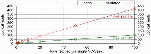
I’ve also fitted linear equations in the chart to see how the slope differs. The heap table matches the theoretic figures pretty closely (3 + 1 per row) but we see “only” four logical reads per row with the clustered index—not the five we would have expected from just fetching one and two rows.
Who cares about logical reads anyway
Logical reads are a fine benchmark because it yields reproducible results—independent of the current state of caches or other work done on the system. However, the above chart is still a very theoretic figure. Four times as many logical reads does not automatically mean four times as slow. In all reality you’ll have a large part of the clustered index in the cache—at least the first few B-tree levels. That reduces the impact definitively. To see how it affects the impact, I conducted another test: measuring the execution time when running the queries from the cache. Avoiding disk access is another way to get more or less reproducible figures that can be compared to each other.
Again, I’ve used 1/2/5-steps but started at 10.000 rows—selecting fewer rows was too fast for the timer’s resolution. Selecting more than 200.000 rows took extraordinarily long so that I believe the data didn’t fit into the cache anymore. Hence I stopped collecting data there.
| Rows Fetched | Time (Heap) | Time (Clustered) |
|---|---|---|
| 10.000 | 31 | 78 |
| 20.000 | 47 | 130 |
| 50.000 | 109 | 297 |
| 100.000 | 203 | 624 |
| 200.000 | 390 | 1232 |
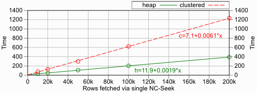
From this test it seems that the “clustered index penalty” on the non-clustered index is more like three times as high as compared to using a heap table.
Notwithstanding these results, is it perfectly possible that the real world caching leads to a “clustered index penalty” outside the here observed range in a production system.
What was the upside of clustered indexes again?
The upside of clustered indexes is that they can deliver subsequent rows quickly when accessed directly (not via a non-clustered index). In other words, they are fast if you use the clustering key to fetch several rows. Remember that the primary key is the clustering key per default. In that case, it means fetching several rows via primary key—with a single query. Hmm. Well, you can’t do that with an equals filter. But how often do you use non-equals filters like > or < on the primary key? Sometimes, maybe, but not that often that it makes sense to optimize the physical table layout for these queries and punish all other indexes with the “clustered index penalty.” That is really insane (IMHO).
Luckily, SQL Server is quite flexible when it comes to clustered indexes. As opposed to MySQL/InnoDB, SQL Server can use any column(s) as clustering key—even non-unique ones. You can choose the clustering key so it catches the most important range scan. Remember that equals predicates (=) can also cause range scans (on non-unique columns). But beware: if you are using long columns and/or many columns as clustering key, they bloat all non-clustered indexes because each row in every non-clustered indexes contains the clustering key as reference to the primary table store. Further, SQL Server makes non-unique clustering keys automatically unique by adding an extra column, which also bloats all non-clustered indexes. Although this bloat will probably not affect the tree depth—thanks to the logarithmic growth of the B-tree—it might still hurt the cache-hit rate. That’s also why the “clustered index penalty” could be outside the range indicated by the tests above—in either way!
Even if you are able to identify the clustering key that brings the most benefit for range scans, the overhead it introduces on the non-clustered indexes can void the gains again. As I said in the intro above, it is just too darn difficult to estimate the overall impact of these effects because the clustering key affects all indexes on the table in a pretty complex way. Therefore, I’m very much in favour of using heap tables if possible and index-only scans when necessary. From this perspective, clustered indexes are just an additional space optimization in case the “clustered index penalty“ isn’t an issue—most importantly if you need only one index that is used for range scans.
Note
Some databases don’t support heap tables at all—most importantly MySQL/MariaDB with InnoDB and the Azure database.
Further there are configurations that can only use the primary key as clustering key—most importantly MySQL/MariaDB with InnoDB and Oracle index-organized tables.
Note that MySQL/MariaDB with InnoDB is on both lists. They don’t offer any alternative for what I referred to as “insane.” MyISAM being no alternative.
Concluding: How many clustered indexes can a SQL Server table have?
To conclude this article, I’d like to demonstrate why it is a bad idea to consider the clustered index as the “silver bullet” that deserves all your thoughts about performance. This demo is simple. Just take a second and think about the following question:
How many clustered indexes can a SQL Server table have?
I love to ask this question in my SQL Server performance trainings. It truly reveals the bad understanding of clustered indexes.
The first answer I get is usually is “one!” Then I ask why I can’t have a second one. Typical response: —silence—. After this article, you already know that a clustered index is not only an index, but also the primary table store. You can’t have two primary table stores. Logical, isn’t it? Next question: Do I need to have a clustered index on every table? Typical response: —silence— or “no” in a doubtful tone. I guess this is when the participants realize that I’m asking trick questions. However, you now know that SQL Server doesn’t need to have a clustered index on every table. In absence of a clustered index, SQL Server uses a heap as table store.
As per definition, the answer to the question is: “at most one.”
And now stop thinking about the clustered index as “silver bullet” and start putting the index-only scan into the focus. For that, I’ll rephrase the question slightly:
How many indexes on a SQL Server table can be queried as fast as a clustered index?
The only change to the original question is that it doesn’t focus on the clustered index as such anymore. Instead it puts your focus on the positive effect you expect from a clustering index. The point in using a clustered index is not just to have a clustered index, it is about improving performance. So, let’s focus on that.
What makes the clustered index fast is that every (direct) access is an index-only scan. So the question essentially boils down to: “how many indexes can support an index-only scan?” And the simple answer is: as many as you like. All you need to do is to add all the required columns to a non-clustered index and *BAM* using it is as fast as though it was a clustered index. That’s what SQL Server’s INCLUDE keyword of the CREATE INDEX statement is for!
Focusing on index-only scans instead of clustered indexes has several advantages:
-
You are not limited to one index. Any index can be as fast as a clustered index.
-
Adding
INCLUDEcolumns to a non-clustered index doesn’t affect anything else than this particular index. There is no penalty that hurts all other indexes! -
You don’t need to add all table columns to a non-clustered index to enable an index-only scan. Just add the columns that are relevant for the query you’d like to tune. That keeps the index small and can thus become even faster than a clustered index.
-
And the best part is: there is no mutual exclusion of index-only scans and clustered indexes. Index-only scans work irrespective of the table storage. You can extend non-clustered indexes for index-only scans even if there is a clustered index. That’s also an easy way to avoid paying the “clustered index penalty” on non-clustered indexes.
Because of the “clustered index penalty” the concept of the index-only scan is even more important when having a clustered index. Really, if there is something like a “silver bullet”, it is the index-only scan—not the clustered index.
If you like my way to explain things, you’ll love SQL Performance Explained.