Вступление
Я читаю статьи о глубоком обучении уже несколько лет, но до недавнего времени не копался и не реализовывал какие-либо модели, используя методы глубокого обучения для себя. Чтобы исправить это, я начал экспериментировать с Deeplearning4J несколько недель назад, но с ограниченным успехом . Я читаю больше книг , учебников для начинающих и учебных пособий, особенно удивительную серию публикаций в блогах Криса Олаха и Денни Брица . Затем, с невероятным временем для меня, Google выпустил TensorFlow к большому волнению. Итак, я решил попробовать, особенно учитывая энтузиазм Делипа Рао — он даже сравнил переход от Theano TensorFlow — ощущение перехода от «Honda Civic к Ferrari».
Вот небольшая прелюдия, прежде чем перейти к моим первоначальным простым исследованиям с TensorFlow. Как известно большинству людей (мы надеемся), глубокое обучение включает в себя идеи, появившиеся много десятилетий назад (реализованные под названиями коннекционизма и нейронных сетей), которые стали масштабными только в последнее десятилетие с появлением более быстрых машин и некоторых алгоритмических инноваций. Я впервые познакомился с ними в классе, который преподавал мой доктор философии Марк Стидман в Университете Пенсильвании в 1997 году. Он особенно интересовался тем, как их можно применить к пониманию языка, о котором он писал в своей статье 1999 года « Connectionist». Обработка предложения в перспективе«. Хотелось бы, чтобы я тогда понял больше об этой теме (и многих других), но опять же, такова природа молодого аспиранта.
Так или иначе, интерес Марка к обработке коннекционистского языка частично возник из-за того, что он был членом диссертационного комитета Джеймса Хендерсона , который завершил свою диссертацию « Анализ на основе описания в сети коннекционистов » в 1994 году. Джеймс работал в Институте исследований в области когнитивных технологий. Наука в Пенне, когда я приехал в 1996 году. Будучи молодым аспирантом, я мало представлял себе, что влечет за собой анализ коннекциониста, и мое понимание от более старших (и гораздо более знающих) студентов было то, что парсеры Джеймса были действительно интересными, но он имел проблемы с масштабированием моделей до более крупных наборов данных — по крайней мере по сравнению с анализаторами, управляемыми данными, которые другие, такие как Майк Коллинз и Адвайт Ратнарпаркистроили в Пенне в середине 1990-х годов. (Примечание: для всех детей, использующих логистическую регрессию для НЛП, вы, вероятно, не знаете, что Adwait был первым, кто применил LR / MaxEnt к нескольким проблемам НЛП в своей диссертации 1998 года « Модели максимальной энтропии для разрешения неоднозначности естественного языка»). «, В котором он продемонстрировал, насколько удивительно это было эффективно для всего, от классификации до пометки части речи и анализа».)
Вернемся к TensorFlow и современности. На прошлой неделе я вылетел из Остина в Вашингтон, округ Колумбия, а накануне полета я скачал TensorFlow, убедился, что все скомпилировано, загрузил необходимые наборы данных и открыл кучу вкладок с учебными пособиями TensorFlow. Моя цель состояла в том, чтобы в самолете запустить учебные пособия, почувствовать поток TensorFlow, а затем внедрить собственные сети для решения некоторых вымышленных задач классификации. Я вышел из упражнения чрезвычайно довольным. Этот пост объясняет, что я сделал, и дает ссылки на код, чтобы это произошло. Моя цель — помочь людям, которые могли бы использовать немного более четкие инструкции и указания, используя полный пример с простыми для понимания данными.Я не буду приводить много примеров кода в этом посте, так как есть несколько учебных пособий, которые уже делают это достаточно хорошо — ценность здесь в простых сквозных реализациях, данных, которые будут сопровождать их, и немного объяснения по пути.
As a preliminary, I recommend going to the excellent TensorFlow documentation, downloading it, and running the first example. If you can do that, you should be able to run the code I’ve provided to go along with this post in my try-tf repository on Github.
Simulated Data
As a researcher who works primarily on empirical methods in natural language processing, my usual tendency is to try new software and ideas out on language data sets, e.g. text classification problems and the like. However, after hanging out with a statistician like James Scott for many years, I’ve come to appreciate the value of using simulated datasets early on to reduce the number of unknowns while getting the basics right. So, when sitting down with TensorFlow, I wanted to try three simulated data sets: linearly separable data, moon data and saturn data. The first is data that linear classifiers can handle easily, while the latter two require the introduction of non-linearities enabled by models like multi-layer neural networks. Here’s what they look like, with brief descriptions.
The linear data has two clusters that can be separated by a diagonal line from top left to bottom right:
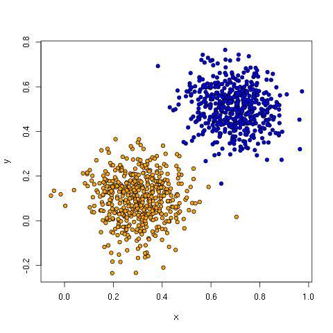
Linear classifiers like perceptrons, logistic regression, linear discriminant analysis, support vector machines and others do well with this kind of data because learning these lines (hyperplanes) is exactly what they do.
The moon data has two clusters in crescent shapes that are tangled up such that no line can keep all the orange dots on one side without also including blue dots.
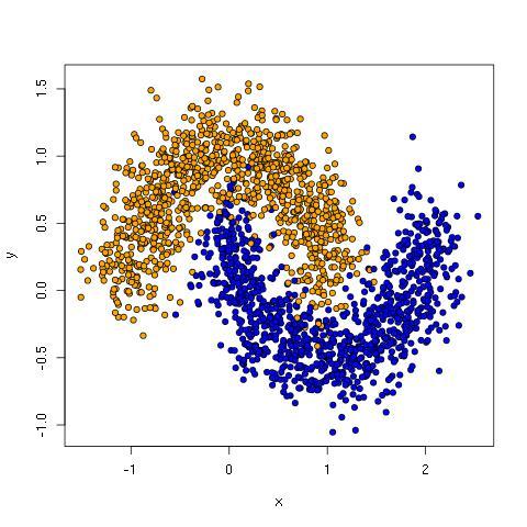
Note: see Implementing a Neural Network from Scratch in Python for a discussion working with the moon data using Theano.
The saturn data has a core cluster representing one class and a ring cluster representing the other.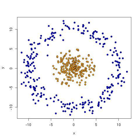
With the saturn data, a line is catastrophically bad. Perhaps the best one can do is draw a line that has all the orange points to one side. This ensures a small, entirely blue side, but it leaves the majority of blue dots in orange terroritory.
Example data has been generated in try-tf/simdata for each of these datasets, including a training set and test set for each. These are for the two dimensional cases visualized above, but you can use the scripts in that directory to generate data with other parameters, including more dimensions, greater variances, etc. See the commented out code for help to visualize the outputs, or adapt plot_data.R, which visualizes 2-d data in CSV format. See the README for instructions.
Related: check out Delip Rao’s post on learning arbitrary lambda expressions.
Softmax Regression
Let’s start with a network that can handle the linear data, which I’ve written in softmax.py. The TensorFlow page has pretty good instructions for how to define a single layer network for MNIST, but no end-to-end code that defines the network, reads in data (consisting of label plus features), trains and evaluates the model. I found writing this to be a good way to familiarize myself with the TensorFlow Python API, so I recommend trying it yourself before looking at my code and then referring to it if you get stuck.
Let’s run it and see what we get.
$ python softmax.py --train simdata/linear_data_train.csv --test simdata/linear_data_eval.csv
Accuracy: 0.99
This performs one pass (epoch) over the training data, so parameters were only updated once per example. 99% is good held-out accuracy, but allowing two training epochs gets us to 100%.
$ python softmax.py --train simdata/linear_data_train.csv --test simdata/linear_data_eval.csv --num_epochs 2
Accuracy: 1.0
There’s a bit of code in softmax.py to handle options and read in data. The most important lines are the ones that define the input data, the model, and the training step. I simply adapted these from the MNIST beginners tutorial, but softmax.py puts it all together and provides a basis for transitioning to the network with a hidden layer discussed later in this post.
To see a little more, let’s turn on the verbose flag and run for 5 epochs.
$ python softmax.py --train simdata/linear_data_train.csv --test simdata/linear_data_eval.csv --num_epochs 5 --verbose True
Initialized!

Training.
0 1 2 3 4 5 6 7 8 9
10 11 12 13 14 15 16 17 18 19
20 21 22 23 24 25 26 27 28 29
30 31 32 33 34 35 36 37 38 39
40 41 42 43 44 45 46 47 48 49

Weight matrix.
[[-1.87038445 1.87038457]
[-2.23716712 2.23716712]]

Bias vector.
[ 1.57296884 -1.57296848]

Applying model to first test instance.
Point = [[ 0.14756215 0.24351828]]
Wx+b = [[ 0.7521798 -0.75217938]]
softmax(Wx+b) = [[ 0.81822371 0.18177626]]

Accuracy: 1.0
Consider first the weights and bias. Intuitively, the classifier should find a separating hyperplane between the two classes, and it probably isn’t immediately obvious how W and b define that. For now, consider only the first column with w1=-1.87038457, w2=-2.23716712 and b=1.57296848. Recall that w1 is the parameter for the `x` dimension and w2 is for the `y` dimension. The separating hyperplane satisfies Wx+b=0; from which we get the standard y=mx+b form.
Wx + b = 0
w1*x + w2*y + b = 0
w2*y = -w1*x – b
y = (-w1/w2)*x – b/w2
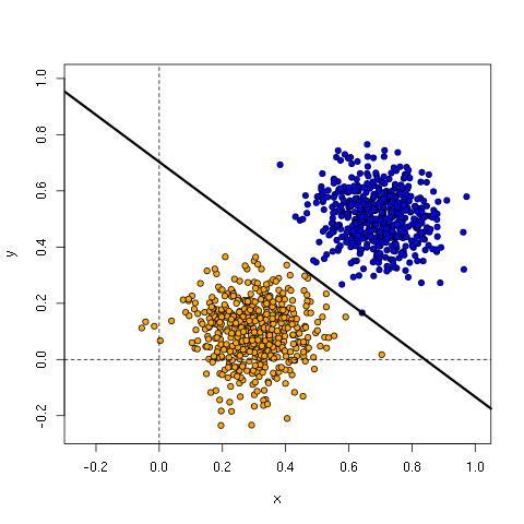
For the parameters learned above, we have the line:
y = -0.8360504*x + 0.7031074
Here’s the plot with the line, showing it is an excellent fit for the training data..
The second column of weights and bias separate the data points at the same place as the first, but mirrored 180 degrees from the first column. Strictly speaking, it is redundant to have two output nodes since a multinomial distribution with n outputs can be represented with n-1 parameters (see section 9.3 of Andrew Ng’s notes on supervised learning for details). Nonetheless, it’s convenient to define the network this way.
Finally, let’s try the softmax network on the moon and saturn data.
python softmax.py --train simdata/moon_data_train.csv --test simdata/moon_data_eval.csv --num_epochs 2
Accuracy: 0.856

$ python softmax.py --train simdata/saturn_data_train.csv --test simdata/saturn_data_eval.csv --num_epochs 2
Accuracy: 0.45
As expected, it doesn’t work very well!
Network With a Hidden Layer
The program hidden.py implements a network with a single hidden layer, and you can set the size of the hidden layer from the command line. Let’s try first with a two-node hidden layer on the moon data.
$ python hidden.py --train simdata/moon_data_train.csv --test simdata/moon_data_eval.csv --num_epochs 100 --num_hidden 2
Accuracy: 0.88
So,that was an improvement over the softmax network. Let’s run it again, exactly the same way.
$ python hidden.py --train simdata/moon_data_train.csv --test simdata/moon_data_eval.csv --num_epochs 100 --num_hidden 2
Accuracy: 0.967
Very different! What we are seeing is the effect of random initialization, which has a large effect on the learned parameters given the small, low-dimensional data we are dealing with here. (The network uses Xavier initialization for the weights.) Let’s try again but using three nodes.
$ python hidden.py --train simdata/moon_data_train.csv --test simdata/moon_data_eval.csv --num_epochs 100 --num_hidden 3
Accuracy: 0.969
If you run this several times, the results don’t vary much and hover around 97%. The additional node increases the representational capacity and makes the network less sensitive to initial weight settings.
Adding more nodes doesn’t change results much — see the WildML post using the moon data for some nice visualizations of the boundaries being learned between the two classes for different hidden layer sizes.
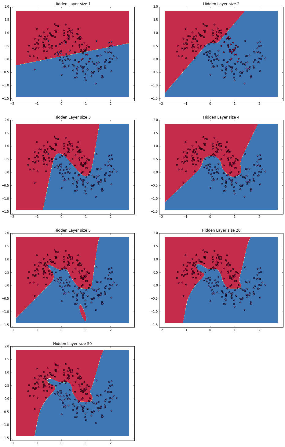
So, a hidden layer does the trick! Let’s see what happens with the saturn data.
$ python hidden.py --train simdata/saturn_data_train.csv --test simdata/saturn_data_eval.csv --num_epochs 50 --num_hidden 2
Accuracy: 0.76
With just two hidden nodes, we already have a substantial boost from the 45% achieved by softmax regression. With 15 hidden nodes, we get 100% accuracy. There is considerable variation from run to run (due to random initialization). As with the moon data, there is less variation as nodes are added. Here’s a plot showing the increase in performance from 1 to 15 nodes, including ten accuracy measurements for each node count.
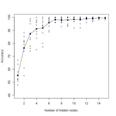
The line through the middle is the average accuracy measurement for each node count.
Initialization and Activation Functions Are Important
My first attempt at doing a network with a hidden layer was to merge what I had done in softmax.py with the network in mnist.py, provided with TensorFlow tutorials. This was a useful exercise to get a better feel for the TensorFlow Python API, and helped me understand the programming model much better. However, I found that I needed to have upwards of 25 or more hidden nodes in order to reliably get >96% accuracy on the moon data.
I then looked back at the WildML moon example and figured something was quite wrong since just three hidden nodes were sufficient there. The differences were that the MNIST example initializes its hidden layers with truncated normals instead of normals divided by the square root of the input size, initializes biases at 0.1 instead of 0 and uses ReLU activations instead of tanh. By switching to Xavier initialization (using Delip’s handy function), 0 biases, and tanh, everything worked as in the WildML example. I’m including my initial version in the repo as truncnorm_hidden.py so that others can see the difference and play around with it. (It turns out that what matters most is the initialization of the weights.)
This is a simple example of what is often discussed with deep learning methods: they can work amazingly well, but they are very sensitive to initialization and choices about the sizes of layers, activation functions, and the influence of these choices on each other. They are a very powerful set of techniques, but they (still) require finesse and understanding, compared to, say, many linear modeling toolkits that can effectively be used as black boxes these days.
Conclusion
I walked away from this exercise very encouraged! I’ve been programming in Scala mostly for the last five years, so it required dusting off my Python (which I taught in my classes at UT Austin from 2005-2011, e.g. Computational Linguistics I and Natural Language Processing), but I found it quite straightforward. Since I work primarily with language processing tasks, I’m perfectly happy with Python since it’s a great language for munging language data into the inputs needed by packages like TensorFlow. Also, Python works well as a DSL for working with deep learning (it seems like there is a new Python deep learning package announced every week these days). It took me less than four hours to go through initial examples, and then build the softmax and hidden networks and apply them to the three data sets. (And a bunch of that time was me remembering how to do things in Python.)
I’m now looking forward to trying deep learning models, especially convnets and LSTM’s, on language and image tasks. I’m also going to go back to my Scala code for trying out Deeplearning4J to see if I can get these simulation examples to run as I’ve shown here with TensorFlow. (I would welcome pull requests if someone else gets to that first!) As a person who works primarily on the JVM, it would be very handy to be able to work with DL4J as well.
After that, maybe I’ll write out the re-occurring rant going on in my head about deep learning not removing the need for feature engineering (as many backpropagandists seem to like to claim), but instead changing the nature of feature engineering, as well as providing a really cool set of new capabilities and tricks.