Этот пост был первоначально написан Стивеном Маллеттом и Дэниелом Куппицем для Аврелия.
«Любопытнее и страннее! воскликнула Алиса (она была настолько удивлена, что на данный момент она совсем забыла, как хорошо говорить по-английски); «Теперь я открываюсь как самый большой телескоп, который когда-либо был!»
— Льюис Кэрролл — Приключения Алисы в стране чудес
 Иногда удивительно видеть, сколько данных доступно. Как и в случае с Алисой и ее внезапным увеличением высоты, в известной истории Льюиса Кэрролла рост данных может происходить довольно быстро, и сразу же появляется возможность создать многомиллиардный граничный граф . К счастью, Titan способен масштабировать до такого размера, и при правильной стратегии загрузки этих данных усилия по разработке могут более быстро перейти к выгодам крупномасштабной аналитики графов.
 Эта статья представляет собой второй выпуск из серии « Полномочия десяти» из двух частей, в которой обсуждаются данные по массовой загрузке в Titan в различных масштабах. Для целей этой серии «масштаб» определяется количеством загружаемых ребер. Как это происходит, стратегии массовой загрузки имеют тенденцию меняться по мере того, как масштаб увеличивается по степеням десяти , что создает запоминающийся способ классификации различных стратегий. В «Части I» этой серии мы рассмотрели стратегии загрузки миллионов и десятков миллионов ребер и сосредоточились на использовании Gremlin для этого. Эта часть серии будет посвящена сотням миллионов и миллиардам ребер и будет посвящена использованию Faunus в качестве инструмента загрузки.
Примечание . В версии Titan 0.5.0 Фаунус будет вовлечен в проект Titan под названием Titan / Hadoop .
100 миллионов
 Как напоминание предшественника этой статьи, загрузка десятков миллионов ребер была лучше всего обработана с помощью BatchGraph . Использование
 BatchGraphможет также быть полезным в сотнях миллионов ребер, предполагая, что время загрузки, связанное с итерацией разработки, не является проблемой. Именно в этот момент решение использовать Фаунуса для загрузки может быть хорошим.
Faunus — это механизм аналитики графов, основанный на Hadoop, и в дополнение к своей роли аналитического инструмента, Faunus также предоставляет способы управления крупномасштабными графами, предоставляя функции, связанные с ETL . Используя преимущества параллельной природы Hadoop, можно сократить время загрузки сотен миллионов кромок по сравнению с подходом с однопоточной загрузкой BatchGraph.
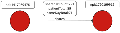
DocGraph набор данных «показывает , как медики команды , чтобы обеспечить уход». DocGraph был представлен в предыдущей части серии Powers of Ten , где использовалась самая маленькая версия набора данных. В качестве быстрого напоминания о содержании этого набора данных напомним, что вершины в этой сети представляют поставщиков медицинских услуг, а ребра — общие взаимодействия между двумя поставщиками. В этом разделе будет использовано «365-дневное окно», состоящее из примерно 1 миллиона вершин и 154 миллионов ребер.
Graphs in the low hundreds of millions of edges, like DocGraph, can often be loaded using a single Hadoop node running in psuedo-distributed mode. In this way, it is possible to have gain the advantage of parallelism, while keeping the configuration complexity and resource requirements as low as possible. In developing this example, a single m2.xlargeEC2 instance was used to host Hadoop and Cassandra in a single-machine cluster. It assumes that the following prerequisites are in place:
- Faunus and Hadoop have been installed as described in the Faunus Getting Started guide.
- Cassandra is installed and running in Local Server Mode.
- Titan has been downloaded and unpacked.
Once the prerequisites have been established, download the DocGraph data set and unpackage it to $FAUNUS_HOME/:
$ curl -L -O http://bit.ly/DocGraph-2012-2013-Days365zip
$ unzip DocGraph-2012-2013-Days365zip
One of the patterns established in the previous Powers of Ten post was the need to always create the Titan Type Definitions first. This step is most directly accomplished by connecting to Cassandra with the Titan Gremlin REPL (i.e. $TITAN_HOME/bin/gremlin.sh) which will automatically establish the Titan keyspace. Place the following code in a file at the root of called $TITAN_HOME/schema.groovy:
g = com.thinkaurelius.titan.core.TitanFactory.open("conf/titan-cassandra.properties")
g.makeKey("npi").dataType(String.class).single().unique().indexed(Vertex.class).make()
sharedTxCount = g.makeKey("sharedTxCount").dataType(Integer.class).make()
patientTotal = g.makeKey("patientTotal").dataType(Integer.class).make()
sameDayTotal = g.makeKey("sameDayTotal").dataType(Integer.class).make()
g.makeLabel("shares").signature(sharedTxCount, patientTotal, sameDayTotal).make()
g.commit()
This file can be executed in the REPL as: gremlin> \. schema.groovy
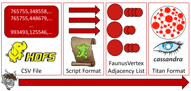
![]() The DocGraph data is formatted as a CSV file, which means that in order to read this data the Faunus input format must be capable of processing that structure. Faunus provides a number of out-of-the-box formats to work with and the one to use in this case is the ScriptInputFormat. This format allows specification of an arbitrary Gremlin script to write a
The DocGraph data is formatted as a CSV file, which means that in order to read this data the Faunus input format must be capable of processing that structure. Faunus provides a number of out-of-the-box formats to work with and the one to use in this case is the ScriptInputFormat. This format allows specification of an arbitrary Gremlin script to write a FaunusVertex, where the FaunusVertex is the object understood by the various output formats that Faunus supports.
The diagram below visualizes the process, where the script defined to the ScriptInputFormat will execute against each line of the CSV file in a parallel fashion, allowing it to parse the line into a resulting FaunusVertex and related edges, forming an adjacency list. That adjacency list can then be written to Cassandra with the TitanCassandraInputFormat.
The following script contains the code to parse the data from the CSV file and will be referred to as $FAUNUS_HOME/NPIScriptInput.groovy
ID_CHARACTERS = ['0'..'9','D'].flatten()
NUM_CHARACTERS = ID_CHARACTERS.size()
deflongencodeId(String id) {
id.inject(0L, { acc, c ->
acc * NUM_CHARACTERS + ID_CHARACTERS.indexOf(c)
})
}
defbooleanread(FaunusVertex vertex, String line) {
def(id1,
id2,
sharedTxCount,
patientTotal,
sameDayTotal) = line.split(',')*.trim()
vertex.reuse(encodeId(id1))
vertex.setProperty("npi", id1)
defedge = vertex.addEdge(Direction.OUT, "shares", encodeId(id2))
edge.setProperty("sharedTxCount", sharedTxCount asInteger)
edge.setProperty("patientTotal", patientTotal asInteger)
edge.setProperty("sameDayTotal", sameDayTotal asInteger)
returntrue
}
 The most important aspect of the code above is the definition of the
 read function at line ten, where the FaunusVertex and a single line from the CSV file are fed. This function processes the CSV line by splitting on the comma separator, setting the property on the supplied FaunusVertex and creating the edge represented by that CSV line. Once the script is created to deal with the input file, attention should be turned to the Faunus properties file (named $FAUNUS_HOME/faunus.properties):
# input graph parameters
faunus.graph.input.format=com.thinkaurelius.faunus.formats.script.ScriptInputFormat
faunus.input.location=docgraph/DocGraph-2012-2013-Days365.csv
faunus.graph.input.script.file=docgraph/NPIScriptInput.groovy
faunus.graph.input.edge-copy.direction=OUT
# output data (graph or statistic) parameters
faunus.graph.output.format=com.thinkaurelius.faunus.formats.titan.cassandra.TitanCassandraOutputFormat
faunus.graph.output.titan.storage.backend=cassandra
faunus.graph.output.titan.storage.hostname=localhost
faunus.graph.output.titan.storage.port=9160
faunus.graph.output.titan.storage.keyspace=titan
faunus.graph.output.titan.storage.batch-loading=true
faunus.graph.output.titan.infer-schema=false
mapred.task.timeout=5400000
mapred.max.split.size=5242880
mapred.reduce.tasks=2
mapred.map.child.java.opts=-Xmx8G
mapred.reduce.child.java.opts=-Xmx8G
mapred.job.reuse.jvm.num.tasks=-1
faunus.sideeffect.output.format=org.apache.hadoop.mapreduce.lib.output.TextOutputFormat
faunus.output.location=output
faunus.output.location.overwrite=true
 The above properties file defines the settings Faunus will use to execute the loading process. Lines two through five specify the input format and properties related to where the source data is. Note that the file locations specified are representative of locations in Hadoop’s distributed file system, HDFS, and not the local file system. Lines eight through fourteen focus on the output format, which is a
 TitanGraph. These settings are mostly standard Titan configurations, prefixed with faunus.graph.output.titan.. As with previous bulk loading examples in Part I of this series, storage.batch-loading is set to true.
It is now possible to execute the load through the Faunus Gremlin REPL, which can be started with, $FAUNUS_HOME/bin/gremlin.sh. The first thing to do is to make sure that the data and script files are available to Faunus in HDFS. Faunus has built-in help for interacting with that distributed file system, allowing for file moves, directory creation and other such functions.
gremlin> hdfs.mkdir("docgraph")
==>null
gremlin> hdfs.copyFromLocal('DocGraph-2012-2013-Days365.csv','docgraph/DocGraph-2012-2013-Days365.csv')
==>null
gremlin> hdfs.copyFromLocal("NPIScriptInput.groovy","docgraph/NPIScriptInput.groovy")
==>null
Now that HDFS has those files available, execute the Faunus job that will load the data as shown below:
gremlin> g = FaunusFactory.open("faunus.properties")
==>faunusgraph[scriptinputformat->titancassandraoutputformat]
gremlin> g._()
13:55:05 INFO mapreduce.FaunusCompiler: Generating job chain: g._()
13:55:05 WARN mapreduce.FaunusCompiler: Using the distribution Faunus job jar: lib/faunus-0.4.2-job.jar
13:55:05 INFO mapreduce.FaunusCompiler: Compiled to 3 MapReduce job(s)
13:55:05 INFO mapreduce.FaunusCompiler: Executing job 1 out of 3: MapSequence[com.thinkaurelius.faunus.formats.EdgeCopyMapReduce.Map, com.thinkaurelius.faunus.formats.EdgeCopyMapReduce.Reduce]
...
17:55:25 INFO input.FileInputFormat: Total input paths to process : 2
17:55:25 INFO mapred.JobClient: Running job: job_201405141319_0004
17:55:26 INFO mapred.JobClient:  map 0% reduce 0%
17:56:23 INFO mapred.JobClient:  map 1% reduce 0%
...
02:06:46 INFO mapred.JobClient:  map 100% reduce 0%
...
18:54:05 INFO mapred.JobClient:  com.thinkaurelius.faunus.formats.BlueprintsGraphOutputMapReduce$Counters
18:54:05 INFO mapred.JobClient:  EDGE_PROPERTIES_WRITTEN=463706751
18:54:05 INFO mapred.JobClient:  EDGES_WRITTEN=154568917
18:54:05 INFO mapred.JobClient:  SUCCESSFUL_TRANSACTIONS=624
...
18:54:05 INFO mapred.JobClient:  SPLIT_RAW_BYTES=77376
At line one, the FaunusGraph instance is created using the docgraph.properties file to configure it. Line three, executes the job given the configuration. The output from the job follows, culminating in EDGES_WRITTEN=154568917, which is the number expected from this dataset.
The decision to utilize Faunus for loading at this scale will generally be balanced against the time of loading and the complexity involved in handling parallelism in a custom way. In other words, BatchGraph and custom parallel loaders might yet be good strategies if time isn’t a big factor or if parallelism can be easily maintained without Hadoop. Of course, using Faunus from the beginning will allow the same load to scale up easily, as converting from a single machine pseudo-cluster, to a high-powered, multi-node cluster isn’t difficult to do and requires no code changes for that to happen.
1 Billion
 In terms of loading mechanics, the approach to loading billions of edges, is not so different from the previous section. The strategy for loading is still Faunus-related, however a single machine psuedo-cluster is likely under-powered for a job of this magnitude. A higher degree of parallelism is required for it to execute in a reasonable time frame. It is also likely that the loading of billions of edges will require some trial-and-error “knob-turning” with respect to Hadoop and the target backend store (e.g. Cassandra).
 The Friendster social network dataset represents a graph with 117 million vertices and 2.5 billion edges. The graph is represented as an edge list, where each line in the CSV file has the out and in vertex represented as a
 long separated by a colon delimiter. Like the previous example with DocGraph, the use of ScriptInputFormat provides the most convenient way to process this file.
In this case, a four node Hadoop cluster was created using m2.4xlarge EC2 instances. Each instance was configured with eight mappers and six reducers, yielding a total of thirty-two mappers and twenty-four reducers in the cluster. Compared to the single machine pseudo-cluster used in the last section, where there were just two mappers and two reducers, this fully distributed cluster has a much higher degree of parallelism. Like the previous section, Hadoop and Cassandra were co-located, where Cassandra was running on each of the four nodes.
As the primary difference between loading data at this scale and the previous one is the use of a fully distributed Hadoop cluster as compared to a pseudo-cluster, this section will dispense with much of the explanation related to execution of the load and specific descriptions of the configurations and scripts involved. The script for processing each line of data in the Friendster dataset looks like this:
importcom.thinkaurelius.faunus.FaunusVertex
importstaticcom.tinkerpop.blueprints.Direction.OUT
defbooleanread(final FaunusVertex v, final String line) {
defparts = line.split(':')
v.reuse(Long.valueOf(parts[0]))
if(parts.size() > 1) {
parts[1].split(',').each({
v.addEdge(OUT, 'friend', Long.valueOf(it))
})
}
returntrue
}
The faunus.properties file isn’t really any different than the previous example except that it now points to Friendster related files in HDFS in the “input format” section. Finally, as with every loading strategy discussed so far, ensure that the Titan schema is established first prior to loading. The job can be executed as follows:
gremlin> hdfs.copyFromLocal("/tmp/FriendsterInput.groovy","FriendsterInput.groovy")
==>null
gremlin> g = FaunusFactory.open("bin/friendster.properties")
==>faunusgraph[scriptinputformat->titancassandraoutputformat]
gremlin> g._()
18:28:46 WARN mapreduce.FaunusCompiler: Using the distribution Faunus job jar: lib/faunus-0.4.4-job.jar
18:28:46 INFO mapreduce.FaunusCompiler: Compiled to 3 MapReduce job(s)
18:28:46 INFO mapreduce.FaunusCompiler: Executing job 1 out of 3: MapSequence[com.thinkaurelius.faunus.formats.EdgeCopyMapReduce.Map, com.thinkaurelius.faunus.formats.EdgeCopyMapReduce.Reduce]
...
18:28:47 INFO input.FileInputFormat: Total input paths to process : 125
18:28:47 INFO mapred.JobClient: Running job: job_201405111636_0005
18:28:48 INFO mapred.JobClient:  map 0% reduce 0%
18:29:39 INFO mapred.JobClient:  map 1% reduce 0%
...
02:06:46 INFO mapred.JobClient:  map 100% reduce 0%
...
02:06:57 INFO mapred.JobClient:  File Input Format Counters
02:06:57 INFO mapred.JobClient:  Bytes Read=79174658355
02:06:57 INFO mapred.JobClient:  com.thinkaurelius.faunus.formats.BlueprintsGraphOutputMapReduce$Counters
02:06:57 INFO mapred.JobClient:  SUCCESSFUL_TRANSACTIONS=15094
02:06:57 INFO mapred.JobClient:  EDGES_WRITTEN=2586147869
02:06:57 INFO mapred.JobClient:  FileSystemCounters
02:06:57 INFO mapred.JobClient:  HDFS_BYTES_READ=79189272471
02:06:57 INFO mapred.JobClient:  FILE_BYTES_WRITTEN=1754590920
...
02:06:57 INFO mapred.JobClient:  Bytes Written=0
The billion edge data load did not introduce any new techniques in loading, but it did show that the same technique used in the hundred million edge scale could scale in a straight-forward manner to billion edge scale without any major changes to the mechanics of loading. Moreover, scaling up Faunus data loads can really just be thought of as introducing more Hadoop nodes to the cluster.
Conclusion
 Over the course of this two post series, a number of strategies have been presented for loading data at different scales. Some patterns, like creating the Titan schema before loading and enabling
 storage.batch-loading, carry through from the smallest graph to the largest and can be thought of as “common strategies”. As there are similarities that can be identified, there are also vast differences ranging from single-threaded loads that take a few seconds to massively parallel loads that can take hours or days. Note that the driver for these variations is the data itself and that aside from “common strategies”, the loading approaches presented can only be thought of as guidelines which must be adapted to the data and the domain.
Complexity of real-world schema will undoubtedly increase as compared to the examples presented in this series. The loading approach may actually consist of several separate load operations, with strategies gathered from each of the sections presented. By understanding all of these loading patterns as a whole, it is possible to tailor the process to the data available, thus enabling the graph exploration adventure.
Acknowledgments
Dr. Vadas Gintautas originally foresaw the need to better document bulk loading strategies and that such strategies seemed to divide themselves nicely in powers of ten.
This post was originally written by Stephen Mallette and Daniel Kuppitz for Aurelius.